Open in Colab: https://colab.research.google.com/github/casangi/graph_viper/blob/master/docs/graph_building_tutorial.ipynb
![]()
GraphVIPER Tutorial
This tutorial provides examples of how GraphVIPER can be used to build Dask graphs by mapping a sub-selection of an xarray.DataTree to Dask graph nodes, followed by a reduction step. The xarray.DataTree used in this tutorial is referred to as a Processing
Set and contains either interferometric visibility data or single dish spectrum data along with relevant metadata. Using the GraphVIPER map and reduce functions can be
thought of as a generalization of xarray.map_blocks that can be applied to a xarray.DataTree. We have designed GraphVIPER so that the graph creation is agnostic of any parallel processing framework: the map and
reduce functions create a dictionary that specifies the graph, and the function generate_dask_workflow converts it into a Dask graph, so we can easily switch to
another technology by writing another variant of generate_dask_workflow. The function generate_dask_workflow creates graphs using dask.delayed.
The following types of mapping are supported:
Partitions defined by any combination of the coordinates in the Processing Set.
More than one MS v4 (xarray.DataTree) can be assigned to a single mapping node.
MS v4 partitions assigned to different nodes can have coordinates that overlap.
The tutorial will cover the following examples:
Frequency Map Reduce: This example explains the concepts of
parallel_coordsandnode_task_data_mappingthat define parallelism.Overlapping Frequency Map Reduce.
Baseline and Frequency Map Reduce.
Time Map Reduce.
GraphVIPER provides improvements over the CNGI prototype:
There is a clear separation between the concurrency layer (GraphVIPER) and the domain layer (science code, AstroVIPER).
The memory backpressure issue was solved by incorporating the loading of data into the compute nodes. An example of the memory backpressure issue is cube imaging where large in-memory image cubes have to be created, which Dask is not aware of, causing Dask to be overeager in loading data from disk into memory. In the future, Dask might provide an alternative solution where graph nodes can be annotated with expected memory usage.
The number of graph nodes has been minimized; this was also solved by incorporating the loading of data into the compute nodes. When Xarray backed Dask datasets are used, a node is created for each data variable, and since Radio Astronomy datasets have numerous data variables, it led to a bloated graph that impacted scaling performance.
Multiple MS v4s in an xarray.DataTree can be processed together with overlap. This cannot be done with current Xarray functionality, such as xarray.map_blocks.
Using a Dask scheduler plugin (
ViperGraphPluginin toolviper), task priorities can be adjusted for the load → map → reduce graph pattern so that only one on-disk chunk group is resident in memory at a time and reductions collapse level by level with minimal memory overhead (see the experimental Data Loading Layer and Scheduler Plugin sections at the end of this tutorial).Data can be cached to a compute node’s local disk when multiple passes over larger-than-memory data have to be done. This reduces clustered file system or binary object store access (an experimental mechanism provided by toolviper and the map function; see the Local Disk Caching section at the end of this tutorial).
Install GraphVIPER
[1]:
import os
import dask
import toolviper

import numpy as np

from importlib.metadata import version

try:
    import graphviper

    print("GraphVIPER version", version("graphviper"), "already installed.")
except ImportError as e:
    print(e)
    print("Installing GraphVIPER")

    os.system("pip install graphviper")

    import graphviper

    print("GraphVIPER version", version("graphviper"), " installed.")
GraphVIPER version 0.0.44 already installed.
Setup Dask Cluster
To simplify things we are going to start off by just using a single process (everything will run in serial).
[2]:
# Code to start a Dask cluster with two workers and 1 thread each.
from toolviper.dask.client import local_client

# viper_client = local_client(cores=2, memory_limit="4GB",autorestrictor=True)
viper_client = local_client(serial_execution=True)
viper_client
[2026-07-08 17:13:31,192]  WARNING      client:  It is recommended that the local cache directory be set using the dask_local_dir parameter.
[2026-07-08 17:13:31,193]     INFO      client:  Running client in synchronous mode.
Download and Convert Dataset
[3]:
toolviper.utils.data.download(file="Antennae_North.cal.lsrk.split.ms")

from xradio.measurement_set.convert_msv2_to_processing_set import convert_msv2_to_processing_set

# The chunksize on disk. Chunksize can be specified for any of the following dimensions :
# time, baseline_id (interferometer) / antenna_id (single dish), frequency, and polarization.
chunks_on_disk = {"frequency": 3}
infile = "Antennae_North.cal.lsrk.split.ms"
outfile = "Antennae_North.cal.lsrk.split.ps.zarr"
convert_msv2_to_processing_set(
    in_file=infile,
    out_file=outfile,
    parallel_mode="none",
    persistence_mode="w",
    main_chunksize=chunks_on_disk,
)
[2026-07-08 17:13:31,202]     INFO      client:  Initializing download...
[2026-07-08 17:13:31,204]     INFO      client:  File already exists: /Users/jsteeb/Dropbox/viper_dev/graphviper/docs/Antennae_North.cal.lsrk.split.ms
[2026-07-08 17:13:31,733]     INFO      client:  Updated partition scheme used: ['DATA_DESC_ID', 'OBS_MODE', 'OBSERVATION_ID']
[2026-07-08 17:13:31,738]     INFO      client:  Selected 4 partitions out of 4
[2026-07-08 17:13:31,738]     INFO      client:  OBSERVATION_ID [0], DDI [0], STATE [23, 24, 25, 30, 31, 32, 33, 34, 37], FIELD [0, 1, 2], SCAN [9, 17, 21, 25], EPHEMERIS [None]
[2026-07-08 17:13:32,719]     INFO      client:  OBSERVATION_ID [1], DDI [0], STATE [23, 24, 25, 30, 31, 32, 33, 34, 37], FIELD [0, 1, 2], SCAN [26, 34, 38, 42], EPHEMERIS [None]
[2026-07-08 17:13:33,221]     INFO      client:  OBSERVATION_ID [2], DDI [0], STATE [32, 33, 34], FIELD [0, 1, 2], SCAN [43], EPHEMERIS [None]
[2026-07-08 17:13:33,620]     INFO      client:  OBSERVATION_ID [3], DDI [0], STATE [39, 40, 41, 46, 47, 48, 49, 50, 53], FIELD [0, 1, 2], SCAN [48, 56, 60, 64], EPHEMERIS [None]
Inspect the Processing Set
The open_processing_set is a lazy function: the data variables are opened as Dask arrays and are not loaded into memory, while the dimension coordinates and attributes are loaded (the load_processing_set will load everything into memory). Note that a Processing
Set does not have to be used with GraphVIPER, and any dictionary of xarray.Datasets can be used.
[4]:
import pandas as pd

pd.options.display.max_colwidth = 100
ps_store = "Antennae_North.cal.lsrk.split.ps.zarr"

from xradio.measurement_set import open_processing_set

fields = None
ps_xdt = open_processing_set(
    ps_store="Antennae_North.cal.lsrk.split.ps.zarr",
    scan_intents=["OBSERVE_TARGET#ON_SOURCE"],
)
display(ps_xdt.xr_ps.summary())
| name | scan_intents | shape | execution_block_UID | polarization | scan_name | spw_name | spw_intents | field_name | source_name | line_name | field_coords | session_reference_UID | scheduling_block_UID | project_UID | start_frequency | end_frequency | |
|---|---|---|---|---|---|---|---|---|---|---|---|---|---|---|---|---|---|
| 0 | Antennae_North.cal.lsrk.split_0 | [OBSERVE_TARGET#ON_SOURCE] | (50, 45, 8, 2) | uid://A002/X1ff7b0/Xb | [XX, YY] | [17, 21, 25, 9] | spw_0 | [UNSPECIFIED] | [NGC4038 - Antennae North_0, NGC4038 - Antennae North_1, NGC4038 - Antennae North_2] | [NGC4038 - Antennae North_0] | [] | Multi-Phase-Center | --- | uid://A002/X1fd4e7/X64d | T.B.D. | 3.439281e+11 | 3.440067e+11 |
| 1 | Antennae_North.cal.lsrk.split_1 | [OBSERVE_TARGET#ON_SOURCE] | (50, 55, 8, 2) | uid://A002/X207fe4/X3a | [XX, YY] | [26, 34, 38, 42] | spw_0 | [UNSPECIFIED] | [NGC4038 - Antennae North_0, NGC4038 - Antennae North_1, NGC4038 - Antennae North_2] | [NGC4038 - Antennae North_0] | [] | Multi-Phase-Center | --- | uid://A002/X1fd4e7/X64d | T.B.D. | 3.439281e+11 | 3.440067e+11 |
| 2 | Antennae_North.cal.lsrk.split_2 | [OBSERVE_TARGET#ON_SOURCE] | (15, 55, 8, 2) | uid://A002/X207fe4/X3b9 | [XX, YY] | [43] | spw_0 | [UNSPECIFIED] | [NGC4038 - Antennae North_0, NGC4038 - Antennae North_1, NGC4038 - Antennae North_2] | [NGC4038 - Antennae North_0] | [] | Multi-Phase-Center | --- | uid://A002/X1fd4e7/X64d | T.B.D. | 3.439281e+11 | 3.440067e+11 |
| 3 | Antennae_North.cal.lsrk.split_3 | [OBSERVE_TARGET#ON_SOURCE, CALIBRATE_WVR#ON_SOURCE] | (50, 77, 8, 2) | uid://A002/X2181fb/X49 | [XX, YY] | [48, 56, 60, 64] | spw_0 | [UNSPECIFIED] | [NGC4038 - Antennae North_0, NGC4038 - Antennae North_1, NGC4038 - Antennae North_2] | [NGC4038 - Antennae North_0] | [] | Multi-Phase-Center | --- | uid://A002/X1fd4e7/X64d | T.B.D. | 3.439281e+11 | 3.440067e+11 |
Inspect a single MS v4
The xarray.DataTrees within a Processing Set are called Measurement Set v4 (MS v4).
[5]:
ms_xds = ps_xdt[
    "Antennae_North.cal.lsrk.split_0"
]

ms_xds
[5]:
<xarray.DataTree 'Antennae_North.cal.lsrk.split_0'>
Group: /Antennae_North.cal.lsrk.split_0
│   Dimensions:                     (time: 50, baseline_id: 45, frequency: 8,
│                                    polarization: 2, uvw_label: 3)
│   Coordinates:
│     * time                        (time) float64 400B 1.307e+09 ... 1.307e+09
│       field_name                  (time) <U46 9kB dask.array<chunksize=(50,), meta=np.ndarray>
│       scan_name                   (time) <U21 4kB dask.array<chunksize=(50,), meta=np.ndarray>
│     * baseline_id                 (baseline_id) int64 360B 0 1 2 3 ... 41 42 43 44
│       baseline_antenna1_name      (baseline_id) <U9 2kB dask.array<chunksize=(45,), meta=np.ndarray>
│       baseline_antenna2_name      (baseline_id) <U9 2kB dask.array<chunksize=(45,), meta=np.ndarray>
│     * frequency                   (frequency) float64 64B 3.439e+11 ... 3.44e+11
│     * polarization                (polarization) <U2 16B 'XX' 'YY'
│     * uvw_label                   (uvw_label) <U1 12B 'u' 'v' 'w'
│   Data variables:
│       EFFECTIVE_INTEGRATION_TIME  (time, baseline_id) float64 18kB dask.array<chunksize=(50, 45), meta=np.ndarray>
│       FLAG                        (time, baseline_id, frequency, polarization) bool 36kB dask.array<chunksize=(50, 45, 3, 2), meta=np.ndarray>
│       TIME_CENTROID               (time, baseline_id) float64 18kB dask.array<chunksize=(50, 45), meta=np.ndarray>
│       UVW                         (time, baseline_id, uvw_label) float64 54kB dask.array<chunksize=(50, 45, 3), meta=np.ndarray>
│       VISIBILITY                  (time, baseline_id, frequency, polarization) complex64 288kB dask.array<chunksize=(50, 45, 3, 2), meta=np.ndarray>
│       WEIGHT                      (time, baseline_id, frequency, polarization) float32 144kB dask.array<chunksize=(50, 45, 3, 2), meta=np.ndarray>
│   Attributes:
│       schema_version:    4.0.0
│       creator:           {'software_name': 'xradio', 'version': '1.2.2'}
│       creation_date:     2026-07-08T21:13:31.761865+00:00
│       type:              visibility
│       data_groups:       {'base': {'correlated_data': 'VISIBILITY', 'flag': 'FL...
│       observation_info:  {'observer': ['Unknown'], 'release_date': '1858-11-17T...
│       processor_info:    {'type': 'CORRELATOR', 'sub_type': 'ALMA_CORRELATOR_MO...
├── Group: /Antennae_North.cal.lsrk.split_0/antenna_xds
│       Dimensions:                 (antenna_name: 10, cartesian_pos_label: 3,
│                                    receptor_label: 2)
│       Coordinates:
│         * antenna_name            (antenna_name) <U9 360B 'DV02_A015' ... 'PM03_J504'
│           mount                   (antenna_name) <U6 240B dask.array<chunksize=(10,), meta=np.ndarray>
│           station_name            (antenna_name) <U4 160B dask.array<chunksize=(10,), meta=np.ndarray>
│           telescope_name          (antenna_name) <U4 160B dask.array<chunksize=(10,), meta=np.ndarray>
│         * cartesian_pos_label     (cartesian_pos_label) <U1 12B 'x' 'y' 'z'
│         * receptor_label          (receptor_label) <U5 40B 'pol_0' 'pol_1'
│           polarization_type       (antenna_name, receptor_label) <U1 80B dask.array<chunksize=(10, 2), meta=np.ndarray>
│       Data variables:
│           ANTENNA_DISH_DIAMETER   (antenna_name) float64 80B dask.array<chunksize=(10,), meta=np.ndarray>
│           ANTENNA_POSITION        (antenna_name, cartesian_pos_label) float64 240B dask.array<chunksize=(10, 3), meta=np.ndarray>
│           ANTENNA_RECEPTOR_ANGLE  (antenna_name, receptor_label) float64 160B dask.array<chunksize=(10, 2), meta=np.ndarray>
│       Attributes:
│           type:                    antenna
│           relocatable_antennas:    True
│           overall_telescope_name:  ALMA
├── Group: /Antennae_North.cal.lsrk.split_0/field_and_source_base_xds
│       Dimensions:                       (field_name: 3, sky_dir_label: 2)
│       Coordinates:
│         * field_name                    (field_name) <U46 552B 'NGC4038 - Antennae ...
│           source_name                   (field_name) <U46 552B dask.array<chunksize=(3,), meta=np.ndarray>
│         * sky_dir_label                 (sky_dir_label) <U3 24B 'ra' 'dec'
│       Data variables:
│           FIELD_PHASE_CENTER_DIRECTION  (field_name, sky_dir_label) float64 48B dask.array<chunksize=(3, 2), meta=np.ndarray>
│           SOURCE_DIRECTION              (field_name, sky_dir_label) float64 48B dask.array<chunksize=(3, 2), meta=np.ndarray>
│       Attributes:
│           type:     field_and_source
└── Group: /Antennae_North.cal.lsrk.split_0/weather_xds
        Dimensions:              (station_name: 2, time_weather: 259,
                                  cartesian_pos_label: 3)
        Coordinates:
          * station_name         (station_name) <U10 80B 'Station_11' 'Station_12'
          * time_weather         (time_weather) float64 2kB 1.307e+09 ... 1.307e+09
          * cartesian_pos_label  (cartesian_pos_label) <U1 12B 'x' 'y' 'z'
        Data variables:
            DEW_POINT            (station_name, time_weather) float64 4kB dask.array<chunksize=(2, 259), meta=np.ndarray>
            PRESSURE             (station_name, time_weather) float64 4kB dask.array<chunksize=(2, 259), meta=np.ndarray>
            REL_HUMIDITY         (station_name, time_weather) float64 4kB dask.array<chunksize=(2, 259), meta=np.ndarray>
            STATION_POSITION     (station_name, cartesian_pos_label) float64 48B dask.array<chunksize=(2, 3), meta=np.ndarray>
            TEMPERATURE          (station_name, time_weather) float64 4kB dask.array<chunksize=(2, 259), meta=np.ndarray>
            WIND_DIRECTION       (station_name, time_weather) float64 4kB dask.array<chunksize=(2, 259), meta=np.ndarray>
            WIND_SPEED           (station_name, time_weather) float64 4kB dask.array<chunksize=(2, 259), meta=np.ndarray>
        Attributes:
type: weatherNomenclature
input_data: A dictionary of xarray.Datasets or a Processing Set (xarray.DataTree).n_datasets: The number of xarray.Datasets in the input_data.i_dim: The \(\text{i}^{\text{th}}\) dimension name.n_dims: The number of dimensions over which parallelism will occur.n_dim_i_chunks: Number of chunks into which the dimension coordinatedim_ihas been divided.n_nodes: Number of nodes in the mapping stage of a MapReduce graph._{}: If curly brackets are preceded by an underscore, it indicates a subscript and not a dictionary value.
How Graph Parallelism is Specified: parallel_coords
The parallel_coords is a dictionary where the keys are dimensions over which parallelism will occur and can be any of the dimension coordinate names present in the input data. For the MS v4 xarray.Dataset, the options include time, baseline_id (interferometer) / antenna_id (single dish), frequency, and polarization. Each dimension coordinate name is associated with a dictionary that describes the data selection for
that dimension in each node of the mapping stage of the graph.
The structure of the parallel_coordinates:
parallel_coords = {
    dim_0: {
        'data': 1D list/np.ndarray of Number,
        'data_chunks': {
            0 : 1D list/np.ndarray of Number,
            ⋮
            n_dim_0_chunks-1 : ...,
        }
        'data_chunk_edges': 1D list/np.ndarray of Number,
        'dims': (dim_0,),
        'attrs': measure attribute,
    }
    ⋮
    dim_{n_dims-1}: ...
}
The dim_i dictionaries keys have the following meanings:
data: An array containing all the coordinate values associated with that dimension. These values do not necessarily have to match the values in the coordinates of the input data, as those are interpolated onto these values. The minimum and maximum values can be respectively larger or smaller than the values in the coordinates of individual xarray.Datasets; this will simply exclude that data from being processed. It’s important to note that theparallel_coordsand the input data coordinates must have the same measures attributes (reference frame, units, etc.).data_chunks: A dictionary where the values are chunks of the data and the keys are integers. This chunking determines the parallelism of the graph. The values in the chunks can overlap.data_chunks_edges: An array with the start and end values of each chunk.dims: The dimension coordinate name.attrs: TheXRADIOmeasures attributes of the data (refer to XRADIO documentation).
The combinations of all the chunks in parallel_coords determine the parallelism of the graph. For example, if you have parallel_coords with 5 time and 3 frequency chunks, you would have 15-way parallelism (5x3).
This description may seem somewhat convoluted, but the following examples should help clarify things.
Frequency Map Reduce
Create Parallel Coordinates
GraphVIPER offers a convenient function, make_parallel_coord, that converts any XRADIO measures to a parallel_coord. In this case, we will use the frequency coordinate of one of the datasets in the Processing
Set. It’s worth noting that all datasets in this Processing Set have the same frequency coordinates but differing time coordinates. This is the case because they represent the same spectral window but different fields in a Mosaic observation.
[6]:
from graphviper.graph_tools.coordinate_utils import make_parallel_coord

parallel_coords = {}
n_chunks = 3
parallel_coords["frequency"] = make_parallel_coord(
    coord=ms_xds.frequency, n_chunks=n_chunks
)

toolviper.utils.display.DataDict.html(parallel_coords["frequency"])
[6]:
data_chunks
data_chunk_slices
attrs
reference_frequency
attrs
channel_width
attrs
The display of the frequency parallel_coords clearly shows how the data was split into 3 chunks. All the chunks must have the same number of values, except the last chunk, which can have fewer. GraphVIPER also has convenience functions that can create frequency and
time coordinate measures:
[7]:
from graphviper.graph_tools.coordinate_utils import make_frequency_coord

n_chunks = 3

coord = make_frequency_coord(
    freq_start=343928096685.9587,
    freq_delta=11231488.981445312,
    n_channels=8,
    velocity_frame="lsrk",
)
parallel_coords["frequency"] = make_parallel_coord(coord=coord, n_chunks=n_chunks)
toolviper.utils.display.DataDict.html(parallel_coords["frequency"])
[7]:
data_chunks
data_chunk_slices
attrs
Create Node Task Data Mapping
Now, the coordinates in the input data must be mapped onto the parallel_coords. This is achieved using the interpolate_data_coords_onto_parallel_coords function, which produces the node_task_data_mapping. It is a dictionary where each key is a node id of one of the nodes in the mapping stage of the graph.
Structure of node_task_data_mapping:
node_task_data_mapping = {
    0 : {
        'chunk_indices': tuple of int,
        'parallel_dims': (dim_0, ..., dim_{n_dims-1}),
        'data_selection': {
                dataset_name_0: {
                        dim_0: slice,
                        ⋮
                        dim_(n_dims-1): slice
                }
                ⋮
                dataset_name_{n_dataset-1}: ...
        }
        'task_coords':
            dim_0:{
                'data': list/np.ndarray of Number,
                'dims': str,
                'attrs': measure attribute,
            }
            ⋮
            dim_(n_dims-1): ...
        }
    ⋮
    n_nodes-1 : ...
}
Each node_id dictionary has the keys with the following meaning:
chunk_indices: The indices assigned to the data chunks in theparallel_coords. There must be an index for eachparallel_dims.parallel_dims: The dimension coordinates over which parallelism will occur.data_selection: A dictionary where the keys are the names of the datasets in theprocessing_set, and the values are dictionaries with the coordinates and accompanying slices. If a coordinate is not included, all values will be selected.task_coords: The chunk of the parallel_coord that is assigned to this node.
[8]:
from graphviper.graph_tools.coordinate_utils import (
    interpolate_data_coords_onto_parallel_coords,
)

node_task_data_mapping = interpolate_data_coords_onto_parallel_coords(
    parallel_coords, ps_xdt
)

toolviper.utils.display.DataDict.html(node_task_data_mapping)
[8]:
0
data_selection
Antennae_North.cal.lsrk.split_0
Antennae_North.cal.lsrk.split_1
Antennae_North.cal.lsrk.split_2
Antennae_North.cal.lsrk.split_3
task_coords
frequency
attrs
1
data_selection
Antennae_North.cal.lsrk.split_0
Antennae_North.cal.lsrk.split_1
Antennae_North.cal.lsrk.split_2
Antennae_North.cal.lsrk.split_3
task_coords
frequency
attrs
2
data_selection
Antennae_North.cal.lsrk.split_0
Antennae_North.cal.lsrk.split_1
Antennae_North.cal.lsrk.split_2
Antennae_North.cal.lsrk.split_3
task_coords
frequency
attrs
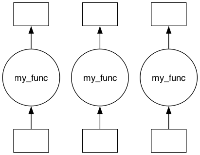
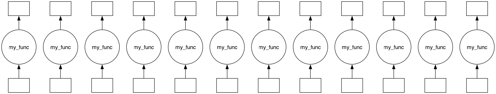
Create a chunk function and map graph
The map function combines a node_task_data_mapping and a node_task to create the map portion of the graph. The node_task may either take a single input_params dictionary (as does the my_func in the example below) or declare an explicit signature whose named parameters are automatically filled from input_params (it is adapted via
make_graph_node_task); it returns a single output. The map function will pass the input_params dictionary to the node_task and add the following items from the node_task_data_mapping:
chunk_indices
parallel_dims
data_selection
task_coords
task_id
If local caching is enabled the following will also be included with the input_params dictionary:
date_time
viper_local_dir
Note that map does not build a Dask graph itself — it returns a plain Python dictionary describing the graph, which `generate_dask_workflow <https://graphviper.readthedocs.io/en/latest/_api/autoapi/graphviper/graph_tools/generate_dask_workflow/index.html#graphviper.graph_tools.generate_dask_workflow.generate_dask_workflow>`__ then converts into a Dask graph (the structure of this dictionary is described just below).
[9]:
#Iff an error is given about graphviz not being installed, please install it using the following command:
# conda install Graphviz

%load_ext autoreload
%autoreload 2

from graphviper.graph_tools.map import map
from graphviper.graph_tools.generate_dask_workflow import generate_dask_workflow

def my_func(input_params):
    toolviper.utils.display.DataDict.html(input_params)

    print("*" * 30)
    return input_params["test_input"]


input_params = {}
input_params["test_input"] = 42

viper_graph = map(
    input_data=ps_xdt,
    node_task_data_mapping=node_task_data_mapping,
    node_task=my_func,
    input_params=input_params,
)

dask_graph = generate_dask_workflow(viper_graph)
dask.visualize(dask_graph, filename="map_graph")
[9]:
The GraphVIPER graph dictionary
Notice that map (and reduce) do not build a Dask graph directly. They return a plain, framework-agnostic Python dictionary — the GraphVIPER graph — that fully describes the work to be done. Only `generate_dask_workflow <https://graphviper.readthedocs.io/en/latest/_api/autoapi/graphviper/graph_tools/generate_dask_workflow/index.html#graphviper.graph_tools.generate_dask_workflow.generate_dask_workflow>`__ turns that dictionary into
`dask.delayed <https://docs.dask.org/en/stable/delayed.html>`__ objects. Because the graph description is decoupled from the execution framework, the same dictionary can instead be handed to another back-end — for example `processes_with_mpi <https://graphviper.readthedocs.io/en/latest/_api/autoapi/graphviper/graph_tools/process_with_mpi/index.html#graphviper.graph_tools.process_with_mpi.processes_with_mpi>`__ — without changing any of the mapping or reduce code.
Immediately after map, the dictionary has a single "map" layer:
viper_graph = {
    "map": {
        "node_task": <callable>,           # the per-node function
        "input_params": [ {...}, ... ],    # one input_params dict per map node
    }
}
reduce appends a "reduce" layer that records how the map outputs are combined (it does not build any Dask nodes itself):
viper_graph["reduce"] = {
    "mode": "tree",        # "tree" | "single_node" | "tree_n"
    "node_task": <callable>,
    "input_params": {...},
    "n_batch": 2,          # inputs combined per reduce node (used by "tree_n")
}
The optional, experimental data-loading layer adds a third "load" layer (plus "load_node_ids" and "relative_data_selections" on the "map" layer); it is covered in the Data Loading Layer section at the end of this tutorial.
The cell below displays this dictionary for the map graph we just built.
[10]:
toolviper.utils.display.DataDict.html(viper_graph)
[10]:
map
[11]:
dask_graph
[11]:
[Delayed('my_func-99645a3d-7a5d-470d-9cd4-954e4f4ae837'),
 Delayed('my_func-8ee29099-cfb5-4316-96c0-a7cc37db86e9'),
 Delayed('my_func-c9310e5d-7103-4525-a520-1cce6bbbfe53')]
Run Map Graph
[12]:
dask.compute(dask_graph)
******************************
******************************
******************************
[12]:
([42, 42, 42],)
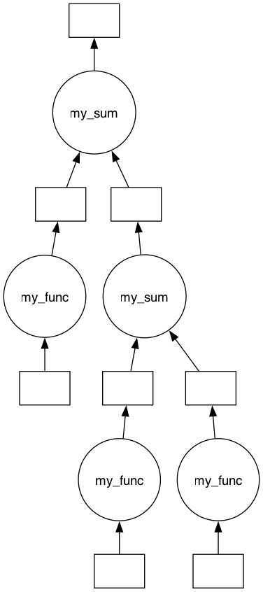
Reduce Graph
The reduce function takes the graph created by the map function and adds a reduce graph that combines the outputs using one of three methods:
single_node: where the output from allmapnodes is sent to a single node,tree: where the outputs are combined using a binary tree reduction.tree_n: where the outputs are combined using a tree reduction in which each reduce node combinesn_batchinputs per layer (n_batch=2reproducestree; a largern_batchyields a shallower tree, trending towardsingle_node).
The function that forms the nodes in the reduce portion of the graph must have two parameters: input_data and input_params. The input_data represents the output from the mapping nodes, while input_params comes from the reduce parameter with the same name.
[13]:
# Single Node Reduce
from graphviper.graph_tools import reduce

def my_sum(graph_inputs, input_params):
    print(graph_inputs)
    return np.sum(graph_inputs / input_params["test_input"])


input_params = {}
input_params["test_input"] = 5
viper_graph_reduce = reduce(
    viper_graph, my_sum, input_params, mode="single_node"
)  # mode "tree","single_node"

print(viper_graph_reduce)

dask_graph_reduce = generate_dask_workflow(viper_graph_reduce)
dask.visualize(dask_graph_reduce)
{'map': {'node_task': <function my_func at 0x1255f4cc0>, 'input_params': [{'test_input': 42, 'chunk_indices': (np.int64(0),), 'parallel_dims': ['frequency'], 'data_selection': {'Antennae_North.cal.lsrk.split_0': {'frequency': slice(np.int64(0), np.int64(3), None)}, 'Antennae_North.cal.lsrk.split_1': {'frequency': slice(np.int64(0), np.int64(3), None)}, 'Antennae_North.cal.lsrk.split_2': {'frequency': slice(np.int64(0), np.int64(3), None)}, 'Antennae_North.cal.lsrk.split_3': {'frequency': slice(np.int64(0), np.int64(3), None)}}, 'task_coords': {'frequency': {'data': array([3.43928097e+11, 3.43939328e+11, 3.43950560e+11]), 'dims': 'frequency', 'attrs': {'units': 'Hz', 'type': 'spectral_coord', 'velocity_frame': 'lsrk'}, 'slice': slice(0, 3, None)}}, 'task_id': 0, 'input_data': None, 'date_time': None}, {'test_input': 42, 'chunk_indices': (np.int64(1),), 'parallel_dims': ['frequency'], 'data_selection': {'Antennae_North.cal.lsrk.split_0': {'frequency': slice(np.int64(3), np.int64(6), None)}, 'Antennae_North.cal.lsrk.split_1': {'frequency': slice(np.int64(3), np.int64(6), None)}, 'Antennae_North.cal.lsrk.split_2': {'frequency': slice(np.int64(3), np.int64(6), None)}, 'Antennae_North.cal.lsrk.split_3': {'frequency': slice(np.int64(3), np.int64(6), None)}}, 'task_coords': {'frequency': {'data': array([3.43961791e+11, 3.43973023e+11, 3.43984254e+11]), 'dims': 'frequency', 'attrs': {'units': 'Hz', 'type': 'spectral_coord', 'velocity_frame': 'lsrk'}, 'slice': slice(3, 6, None)}}, 'task_id': 1, 'input_data': None, 'date_time': None}, {'test_input': 42, 'chunk_indices': (np.int64(2),), 'parallel_dims': ['frequency'], 'data_selection': {'Antennae_North.cal.lsrk.split_0': {'frequency': slice(np.int64(6), np.int64(8), None)}, 'Antennae_North.cal.lsrk.split_1': {'frequency': slice(np.int64(6), np.int64(8), None)}, 'Antennae_North.cal.lsrk.split_2': {'frequency': slice(np.int64(6), np.int64(8), None)}, 'Antennae_North.cal.lsrk.split_3': {'frequency': slice(np.int64(6), np.int64(8), None)}}, 'task_coords': {'frequency': {'data': array([3.43995486e+11, 3.44006717e+11]), 'dims': 'frequency', 'attrs': {'units': 'Hz', 'type': 'spectral_coord', 'velocity_frame': 'lsrk'}, 'slice': slice(6, 8, None)}}, 'task_id': 2, 'input_data': None, 'date_time': None}]}, 'reduce': {'mode': 'single_node', 'node_task': <function my_sum at 0x12554dda0>, 'input_params': {'test_input': 5}, 'n_batch': 2}}
[13]:

[14]:
# Tree Reduce
from graphviper.graph_tools import reduce

def my_sum(graph_inputs, input_params):
    print(graph_inputs)
    return np.sum(graph_inputs) + input_params["test_input"]


input_params = {}
input_params["test_input"] = 5
viper_graph_reduce = reduce(
    viper_graph, my_sum, input_params, mode="tree"
)  # mode "tree","single_node","tree_n"

dask_graph_reduce = generate_dask_workflow(viper_graph_reduce)
dask.visualize(dask_graph_reduce)
[14]:
[15]:
toolviper.utils.display.DataDict.html(viper_graph)
[15]:
map
reduce
input_params
Run Map Reduce Graph
[16]:
dask.compute(dask_graph_reduce)
******************************
******************************
[42, 42]
******************************
[np.int64(89), 42]
[16]:
(np.int64(136),)
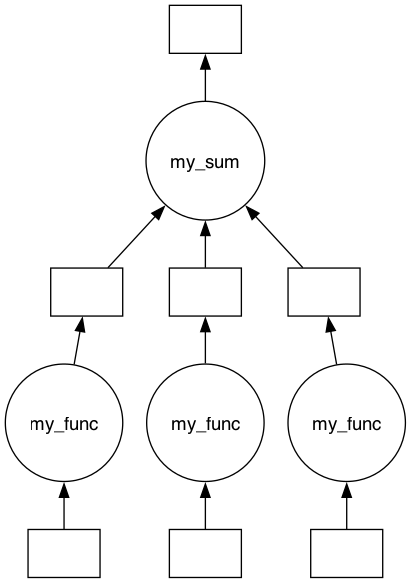
tree_n Reduce (variable-arity tree)
The tree_n mode generalizes tree: each reduce node combines n_batch inputs per layer instead of exactly two. n_batch=2 reproduces the binary tree above, while a larger n_batch produces a shallower tree (fewer layers, more inputs combined per node), trending toward single_node. With the 3-node frequency map graph, n_batch=3 collapses all the outputs in a single reduce layer (whereas the binary tree above used two layers).
[17]:
# `tree_n` reduce: combine `n_batch` inputs per reduce node, layer by layer.
from graphviper.graph_tools import reduce

def my_sum(graph_inputs, input_params):
    return np.sum(graph_inputs) + input_params["test_input"]


viper_graph_reduce_n = reduce(
    viper_graph, my_sum, {"test_input": 5}, mode="tree_n", n_batch=3
)

dask_graph_reduce_n = generate_dask_workflow(viper_graph_reduce_n)
dask.visualize(dask_graph_reduce_n)
[17]:
Overlapping Frequency Map Reduce
Create Parallel Coordinates
[18]:
dask.config.set(scheduler="synchronous")

from xradio.measurement_set import open_processing_set
from IPython.display import HTML, display


ps = open_processing_set(
    ps_store="Antennae_North.cal.lsrk.split.ps.zarr",
    scan_intents=["OBSERVE_TARGET#ON_SOURCE"],
)
ms_xds = ps["Antennae_North.cal.lsrk.split_0"]
n_chunks = 3

parallel_coords = {}
freq_coord = ms_xds.frequency.to_dict()
# Here, we create overlapping data chunks. Currently, there is no convenience function available to assist with this.
freq_coord["data_chunks"] = {
    0: freq_coord["data"][0:4],
    1: freq_coord["data"][3:7],
    2: freq_coord["data"][4:8],
}
parallel_coords["frequency"] = freq_coord

toolviper.utils.display.DataDict.html(parallel_coords["frequency"])
[18]:
attrs
reference_frequency
attrs
channel_width
attrs
coords
frequency
attrs
reference_frequency
attrs
channel_width
attrs
data_chunks
[19]:
ps = open_processing_set(
    ps_store="Antennae_North.cal.lsrk.split.ps.zarr",
    scan_intents=["OBSERVE_TARGET#ON_SOURCE"],
)
ps.xr_ps.summary()
[19]:
| name | scan_intents | shape | execution_block_UID | polarization | scan_name | spw_name | spw_intents | field_name | source_name | line_name | field_coords | session_reference_UID | scheduling_block_UID | project_UID | start_frequency | end_frequency | |
|---|---|---|---|---|---|---|---|---|---|---|---|---|---|---|---|---|---|
| 0 | Antennae_North.cal.lsrk.split_0 | [OBSERVE_TARGET#ON_SOURCE] | (50, 45, 8, 2) | uid://A002/X1ff7b0/Xb | [XX, YY] | [17, 21, 25, 9] | spw_0 | [UNSPECIFIED] | [NGC4038 - Antennae North_0, NGC4038 - Antennae North_1, NGC4038 - Antennae North_2] | [NGC4038 - Antennae North_0] | [] | Multi-Phase-Center | --- | uid://A002/X1fd4e7/X64d | T.B.D. | 3.439281e+11 | 3.440067e+11 |
| 1 | Antennae_North.cal.lsrk.split_1 | [OBSERVE_TARGET#ON_SOURCE] | (50, 55, 8, 2) | uid://A002/X207fe4/X3a | [XX, YY] | [26, 34, 38, 42] | spw_0 | [UNSPECIFIED] | [NGC4038 - Antennae North_0, NGC4038 - Antennae North_1, NGC4038 - Antennae North_2] | [NGC4038 - Antennae North_0] | [] | Multi-Phase-Center | --- | uid://A002/X1fd4e7/X64d | T.B.D. | 3.439281e+11 | 3.440067e+11 |
| 2 | Antennae_North.cal.lsrk.split_2 | [OBSERVE_TARGET#ON_SOURCE] | (15, 55, 8, 2) | uid://A002/X207fe4/X3b9 | [XX, YY] | [43] | spw_0 | [UNSPECIFIED] | [NGC4038 - Antennae North_0, NGC4038 - Antennae North_1, NGC4038 - Antennae North_2] | [NGC4038 - Antennae North_0] | [] | Multi-Phase-Center | --- | uid://A002/X1fd4e7/X64d | T.B.D. | 3.439281e+11 | 3.440067e+11 |
| 3 | Antennae_North.cal.lsrk.split_3 | [OBSERVE_TARGET#ON_SOURCE, CALIBRATE_WVR#ON_SOURCE] | (50, 77, 8, 2) | uid://A002/X2181fb/X49 | [XX, YY] | [48, 56, 60, 64] | spw_0 | [UNSPECIFIED] | [NGC4038 - Antennae North_0, NGC4038 - Antennae North_1, NGC4038 - Antennae North_2] | [NGC4038 - Antennae North_0] | [] | Multi-Phase-Center | --- | uid://A002/X1fd4e7/X64d | T.B.D. | 3.439281e+11 | 3.440067e+11 |
Create Node Task Data Mapping
[20]:
from graphviper.graph_tools.coordinate_utils import (
    interpolate_data_coords_onto_parallel_coords,
)

node_task_data_mapping = interpolate_data_coords_onto_parallel_coords(
    parallel_coords, ps
)

toolviper.utils.display.DataDict.html(node_task_data_mapping)
[20]:
0
data_selection
Antennae_North.cal.lsrk.split_0
Antennae_North.cal.lsrk.split_1
Antennae_North.cal.lsrk.split_2
Antennae_North.cal.lsrk.split_3
task_coords
frequency
attrs
reference_frequency
attrs
channel_width
attrs
1
data_selection
Antennae_North.cal.lsrk.split_0
Antennae_North.cal.lsrk.split_1
Antennae_North.cal.lsrk.split_2
Antennae_North.cal.lsrk.split_3
task_coords
frequency
attrs
reference_frequency
attrs
channel_width
attrs
2
data_selection
Antennae_North.cal.lsrk.split_0
Antennae_North.cal.lsrk.split_1
Antennae_North.cal.lsrk.split_2
Antennae_North.cal.lsrk.split_3
task_coords
frequency
attrs
reference_frequency
attrs
channel_width
attrs
[21]:
{'dims': ('frequency',), 'attrs': {'channel_width': {'attrs': {'type': 'quantity', 'units': 'Hz'}, 'data': 11231488.981445312, 'dims': []}, 'observer': 'lsrk', 'reference_frequency': {'attrs': {'observer': 'lsrk', 'type': 'spectral_coord', 'units': 'Hz'}, 'data': 343928096685.9587, 'dims': []}, 'spectral_window_intents': ['UNSPECIFIED'], 'spectral_window_name': 'spw_0', 'type': 'spectral_coord', 'units': 'Hz'}, 'data': [343928096685.9587, 343939328174.9401, 343950559663.9216, 343961791152.903, 343973022641.88446, 343984254130.8659, 343995485619.84735, 344006717108.8288], 'coords': {'frequency': {'dims': ('frequency',), 'attrs': {'channel_width': {'attrs': {'type': 'quantity', 'units': 'Hz'}, 'data': 11231488.981445312, 'dims': []}, 'observer': 'lsrk', 'reference_frequency': {'attrs': {'observer': 'lsrk', 'type': 'spectral_coord', 'units': 'Hz'}, 'data': 343928096685.9587, 'dims': []}, 'spectral_window_intents': ['UNSPECIFIED'], 'spectral_window_name': 'spw_0', 'type': 'spectral_coord', 'units': 'Hz'},
                                                                                                                                                                                                                                                                                                                                                                                                                                                                                                                                                                                                                           'data': [343928096685.9587, 343939328174.9401, 343950559663.9216, 343961791152.903, 343973022641.88446, 343984254130.8659, 343995485619.84735, 344006717108.8288]}}, 'name': 'frequency',
 'data_chunks': {0: [343928096685.9587, 343939328174.9401, 343950559663.9216, 343961791152.903], 1: [343961791152.903, 343973022641.88446, 343984254130.8659, 343995485619.84735], 2: [343973022641.88446, 343984254130.8659, 343995485619.84735, 344006717108.8288]},
 'data_chunks_edges': [343928096685.9587, 343961791152.903, 343961791152.903, 343995485619.84735, 343973022641.88446, 344006717108.8288]}
[21]:
{'dims': ('frequency',),
 'attrs': {'channel_width': {'attrs': {'type': 'quantity', 'units': 'Hz'},
   'data': 11231488.981445312,
   'dims': []},
  'observer': 'lsrk',
  'reference_frequency': {'attrs': {'observer': 'lsrk',
    'type': 'spectral_coord',
    'units': 'Hz'},
   'data': 343928096685.9587,
   'dims': []},
  'spectral_window_intents': ['UNSPECIFIED'],
  'spectral_window_name': 'spw_0',
  'type': 'spectral_coord',
  'units': 'Hz'},
 'data': [343928096685.9587,
  343939328174.9401,
  343950559663.9216,
  343961791152.903,
  343973022641.88446,
  343984254130.8659,
  343995485619.84735,
  344006717108.8288],
 'coords': {'frequency': {'dims': ('frequency',),
   'attrs': {'channel_width': {'attrs': {'type': 'quantity', 'units': 'Hz'},
     'data': 11231488.981445312,
     'dims': []},
    'observer': 'lsrk',
    'reference_frequency': {'attrs': {'observer': 'lsrk',
      'type': 'spectral_coord',
      'units': 'Hz'},
     'data': 343928096685.9587,
     'dims': []},
    'spectral_window_intents': ['UNSPECIFIED'],
    'spectral_window_name': 'spw_0',
    'type': 'spectral_coord',
    'units': 'Hz'},
   'data': [343928096685.9587,
    343939328174.9401,
    343950559663.9216,
    343961791152.903,
    343973022641.88446,
    343984254130.8659,
    343995485619.84735,
    344006717108.8288]}},
 'name': 'frequency',
 'data_chunks': {0: [343928096685.9587,
   343939328174.9401,
   343950559663.9216,
   343961791152.903],
  1: [343961791152.903,
   343973022641.88446,
   343984254130.8659,
   343995485619.84735],
  2: [343973022641.88446,
   343984254130.8659,
   343995485619.84735,
   344006717108.8288]},
 'data_chunks_edges': [343928096685.9587,
  343961791152.903,
  343961791152.903,
  343995485619.84735,
  343973022641.88446,
  344006717108.8288]}
Map Graph
[22]:
from graphviper.graph_tools.map import map
from xradio.measurement_set import open_processing_set


def my_func(input_params):
    toolviper.utils.display.DataDict.html(input_params)

    print("*" * 30)
    return input_params["test_input"]


input_params = {}
input_params["test_input"] = 42

ps = open_processing_set(
    ps_store="Antennae_North.cal.lsrk.split.ps.zarr",
    scan_intents=["OBSERVE_TARGET#ON_SOURCE"],
)

viper_graph = map(
    input_data=ps,
    node_task_data_mapping=node_task_data_mapping,
    node_task=my_func,
    input_params=input_params,
)

dask_graph = generate_dask_workflow(viper_graph)

dask.visualize(dask_graph, filename="map_graph")
[22]:
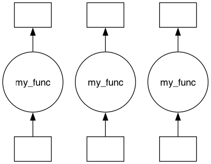
Run Map Graph
[23]:
dask.compute(dask_graph)
******************************
******************************
******************************
[23]:
([42, 42, 42],)
Baseline and Frequency Map Reduce
Create Parallel Coordinates
[24]:
from graphviper.graph_tools.coordinate_utils import make_parallel_coord

dask.config.set(scheduler="synchronous")

from xradio.measurement_set import open_processing_set

intents = ["OBSERVE_TARGET#ON_SOURCE"]
ps = open_processing_set(
    ps_store="Antennae_North.cal.lsrk.split.ps.zarr",
    scan_intents=["OBSERVE_TARGET#ON_SOURCE"],
)

ms_xds = ps["Antennae_North.cal.lsrk.split_0"]

parallel_coords = {}

n_chunks = 4
parallel_coords["baseline_id"] = make_parallel_coord(
    coord=ms_xds.baseline_id, n_chunks=n_chunks
)

n_chunks = 3
parallel_coords["frequency"] = make_parallel_coord(
    coord=ms_xds.frequency, n_chunks=n_chunks
)

toolviper.utils.display.DataDict.html(parallel_coords)
[24]:
baseline_id
data_chunks
data_chunk_slices
attrs
frequency
data_chunks
data_chunk_slices
attrs
reference_frequency
attrs
channel_width
attrs
Create Node Task Data Mapping
[25]:
from graphviper.graph_tools.coordinate_utils import (
    interpolate_data_coords_onto_parallel_coords,
)

node_task_data_mapping = interpolate_data_coords_onto_parallel_coords(
    parallel_coords, ps
)

toolviper.utils.display.DataDict.html(node_task_data_mapping)
[25]:
0
data_selection
Antennae_North.cal.lsrk.split_0
Antennae_North.cal.lsrk.split_1
Antennae_North.cal.lsrk.split_2
Antennae_North.cal.lsrk.split_3
task_coords
baseline_id
attrs
frequency
attrs
reference_frequency
attrs
channel_width
attrs
1
data_selection
Antennae_North.cal.lsrk.split_0
Antennae_North.cal.lsrk.split_1
Antennae_North.cal.lsrk.split_2
Antennae_North.cal.lsrk.split_3
task_coords
baseline_id
attrs
frequency
attrs
reference_frequency
attrs
channel_width
attrs
2
data_selection
Antennae_North.cal.lsrk.split_0
Antennae_North.cal.lsrk.split_1
Antennae_North.cal.lsrk.split_2
Antennae_North.cal.lsrk.split_3
task_coords
baseline_id
attrs
frequency
attrs
reference_frequency
attrs
channel_width
attrs
3
data_selection
Antennae_North.cal.lsrk.split_0
Antennae_North.cal.lsrk.split_1
Antennae_North.cal.lsrk.split_2
Antennae_North.cal.lsrk.split_3
task_coords
baseline_id
attrs
frequency
attrs
reference_frequency
attrs
channel_width
attrs
4
data_selection
Antennae_North.cal.lsrk.split_0
Antennae_North.cal.lsrk.split_1
Antennae_North.cal.lsrk.split_2
Antennae_North.cal.lsrk.split_3
task_coords
baseline_id
attrs
frequency
attrs
reference_frequency
attrs
channel_width
attrs
5
data_selection
Antennae_North.cal.lsrk.split_0
Antennae_North.cal.lsrk.split_1
Antennae_North.cal.lsrk.split_2
Antennae_North.cal.lsrk.split_3
task_coords
baseline_id
attrs
frequency
attrs
reference_frequency
attrs
channel_width
attrs
6
data_selection
Antennae_North.cal.lsrk.split_0
Antennae_North.cal.lsrk.split_1
Antennae_North.cal.lsrk.split_2
Antennae_North.cal.lsrk.split_3
task_coords
baseline_id
attrs
frequency
attrs
reference_frequency
attrs
channel_width
attrs
7
data_selection
Antennae_North.cal.lsrk.split_0
Antennae_North.cal.lsrk.split_1
Antennae_North.cal.lsrk.split_2
Antennae_North.cal.lsrk.split_3
task_coords
baseline_id
attrs
frequency
attrs
reference_frequency
attrs
channel_width
attrs
8
data_selection
Antennae_North.cal.lsrk.split_0
Antennae_North.cal.lsrk.split_1
Antennae_North.cal.lsrk.split_2
Antennae_North.cal.lsrk.split_3
task_coords
baseline_id
attrs
frequency
attrs
reference_frequency
attrs
channel_width
attrs
9
data_selection
Antennae_North.cal.lsrk.split_0
Antennae_North.cal.lsrk.split_1
Antennae_North.cal.lsrk.split_2
Antennae_North.cal.lsrk.split_3
task_coords
baseline_id
attrs
frequency
attrs
reference_frequency
attrs
channel_width
attrs
10
data_selection
Antennae_North.cal.lsrk.split_0
Antennae_North.cal.lsrk.split_1
Antennae_North.cal.lsrk.split_2
Antennae_North.cal.lsrk.split_3
task_coords
baseline_id
attrs
frequency
attrs
reference_frequency
attrs
channel_width
attrs
11
data_selection
Antennae_North.cal.lsrk.split_0
Antennae_North.cal.lsrk.split_1
Antennae_North.cal.lsrk.split_2
Antennae_North.cal.lsrk.split_3
task_coords
baseline_id
attrs
frequency
attrs
reference_frequency
attrs
channel_width
attrs
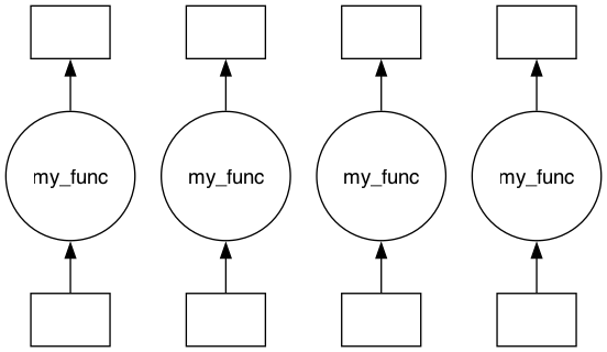
Map Graph
[26]:
from graphviper.graph_tools.map import map

def my_func(input_params):
    toolviper.utils.display.DataDict.html(input_params)

    print("*" * 30)
    return input_params["test_input"]


# ['test_input', 'input_data_name', 'viper_local_dir', 'date_time', 'data_sel', 'chunk_coords', 'chunk_indx', 'chunk_id', 'parallel_dims']
input_params = {}
input_params["test_input"] = 42

viper_graph = map(
    input_data=ps,
    node_task_data_mapping=node_task_data_mapping,
    node_task=my_func,
    input_params=input_params,
)

dask_graph = generate_dask_workflow(viper_graph)
dask.visualize(dask_graph, filename="map_graph")
[26]:
Run Map Graph
[27]:
dask.compute(dask_graph)
******************************
******************************
******************************
******************************
******************************
******************************
******************************
******************************
******************************
******************************
******************************
******************************
[27]:
([42, 42, 42, 42, 42, 42, 42, 42, 42, 42, 42, 42],)
Time Map Reduce
In this example the parallel coordinate is deliberately built from the time coordinates of only three of the four MS v4s in the Processing Set (split_0, split_1, and split_2). The fourth, split_3, belongs to a later execution block whose time range does not overlap the combined time range of the other three. Because all of its time values fall outside the parallel_coords, all of ``split_3``’s data is excluded from the graph: it does not appear in the
data_selection of any node in the node_task_data_mapping below. This demonstrates how the parallel_coords also act as a data selection — any data outside their range is silently excluded from processing. To process all four MS v4s, the time coordinates of all four would have to be combined when constructing the parallel coordinate.
Create Parallel Coordinates
[28]:
from graphviper.graph_tools.coordinate_utils import make_parallel_coord

dask.config.set(scheduler="synchronous")

from xradio.measurement_set import open_processing_set

intents = ["OBSERVE_TARGET#ON_SOURCE"]
ps = open_processing_set(
    ps_store="Antennae_North.cal.lsrk.split.ps.zarr",
    scan_intents=["OBSERVE_TARGET#ON_SOURCE"],
)
ms_xds = ps["Antennae_North.cal.lsrk.split_0"]

parallel_coords = {}

import xarray as xr
import numpy as np

t0, t1, t2 = (ps["Antennae_North.cal.lsrk.split_1"].time, ps["Antennae_North.cal.lsrk.split_0"].time, ps["Antennae_North.cal.lsrk.split_2"].time)
time_coord = xr.concat([t0, t1, t2], dim="time").sortby("time").to_dict()
n_chunks = 4
parallel_coords["time"] = make_parallel_coord(coord=time_coord, n_chunks=n_chunks)

toolviper.utils.display.DataDict.html(parallel_coords["time"])
[28]:
data_chunks
data_chunk_slices
attrs
integration_time
attrs
Create Node Task Data Mapping
Note that Antennae_North.cal.lsrk.split_3 does not appear in the data_selection of any node below — its time range lies entirely outside the parallel coordinates, so none of its data will be processed.
[29]:
from graphviper.graph_tools.coordinate_utils import (
    interpolate_data_coords_onto_parallel_coords,
)

node_task_data_mapping = interpolate_data_coords_onto_parallel_coords(
    parallel_coords, ps
)

toolviper.utils.display.DataDict.html(node_task_data_mapping)
[29]:
0
data_selection
Antennae_North.cal.lsrk.split_0
task_coords
time
attrs
integration_time
attrs
1
data_selection
Antennae_North.cal.lsrk.split_0
Antennae_North.cal.lsrk.split_1
task_coords
time
attrs
integration_time
attrs
2
data_selection
Antennae_North.cal.lsrk.split_1
task_coords
time
attrs
integration_time
attrs
3
data_selection
Antennae_North.cal.lsrk.split_1
Antennae_North.cal.lsrk.split_2
task_coords
time
attrs
integration_time
attrs
Map Graph
[30]:
import dask

from graphviper.graph_tools.map import map

def my_func(input_params):
    toolviper.utils.display.DataDict.html(input_params)

    print("*" * 30)
    return input_params["test_input"]


# ['test_input', 'input_data_name', 'viper_local_dir', 'date_time', 'data_sel', 'chunk_coords', 'chunk_indx', 'chunk_id', 'parallel_dims']
input_params = {}
input_params["test_input"] = 42

viper_graph = map(
    input_data=ps,
    node_task_data_mapping=node_task_data_mapping,
    node_task=my_func,
    input_params=input_params,
)

dask_graph = generate_dask_workflow(viper_graph)
dask.visualize(dask_graph, filename="map_graph")
[30]:
Run Map Graph
[31]:
dask.compute(dask_graph)
******************************
******************************
******************************
******************************
[31]:
([42, 42, 42, 42],)
Data Loading Layer
This is experimental
In the examples above each map node is assigned only its own small slice of the input data (its data_selection), which the node task reads from disk. This is efficient when the on-disk zarr chunk size matches the map partition size exactly, but in practice the two rarely align.
Example: a zarr store with 200 frequency channels per chunk and a map graph with 2 channels per task will cause 100 map nodes to open the same compressed chunk on disk — decompressing it 100 times instead of once.
The data loading layer solves this by inserting shared load nodes between the input store and the map nodes:
disk store
    │
 [load node]  ← reads one full zarr chunk (e.g. 200 channels), shared by
    │  │         all map tasks that fall inside that chunk
    │  │
 [prepare]  [prepare]  …  ← sub-selects each task's 2-channel slice (in memory)
    │           │
 [map task] [map task] …  ← receives pre-loaded data via input_params["input_data"]
Only the dimensions listed in disk_chunk_sizes are coalesced this way; all other dimensions are handled exactly as before.
Detect Native Disk Chunk Sizes
get_disk_chunk_sizes inspects the dask chunk metadata on the data variables of a lazily-opened zarr store to find the native compression chunk size for each parallel dimension. Data variables — rather than coordinates — are inspected because xarray always loads dimension coordinates eagerly into memory as numpy-backed indexes, so only the lazily loaded data variables carry the on-disk chunk information.
Recall that this tutorial’s Processing Set was written with main_chunksize = {"frequency": 3}, so the native chunk size along frequency is 3 (i.e. the 8 channels are stored in 3 zarr chunks).
[32]:
from graphviper.graph_tools.coordinate_utils import (
    make_parallel_coord,
    interpolate_data_coords_onto_parallel_coords,
    get_disk_chunk_sizes,
)
from graphviper.graph_tools.map import map
from graphviper.graph_tools.generate_dask_workflow import generate_dask_workflow

# Re-open the processing set lazily so the data variables are dask arrays
# that carry the native on-disk (zarr) chunk sizes.
from xradio.measurement_set import open_processing_set

ps_xdt = open_processing_set(
    ps_store=ps_store,
    scan_intents=["OBSERVE_TARGET#ON_SOURCE"],
)

# Use more map tasks than zarr chunks to create a mismatch (realistic scenario).
# Note: requesting 9 chunks of an 8-channel axis yields 8 single-channel chunks.
n_chunks = 9
parallel_coords = {}
parallel_coords["frequency"] = make_parallel_coord(
    coord=ms_xds.frequency, n_chunks=n_chunks
)
n_map_tasks = len(parallel_coords["frequency"]["data_chunks"])

disk_chunk_sizes = get_disk_chunk_sizes(ps_xdt, parallel_coords)
first_ms_xdt = ps_xdt[list(ps_xdt.children)[0]]
n_zarr_chunks = {
    dim: int(np.ceil(len(first_ms_xdt[dim]) / size))
    for dim, size in disk_chunk_sizes.items()
}
print("Native on-disk chunk sizes:", disk_chunk_sizes)
print(f"Map tasks: {n_map_tasks}   |   Zarr chunks per dim: {n_zarr_chunks}")
Native on-disk chunk sizes: {'frequency': 3}
Map tasks: 8   |   Zarr chunks per dim: {'frequency': 3}
Define a Load Task
The load task is an ordinary Python function called once per unique disk chunk. It receives load_params containing:
"input_data_store"— path to the zarr store"data_selection"—{xds_name: {dim: slice}}at disk-chunk granularityany extra keys passed via
load_node_input_params
It must return a dict-like mapping of dataset names to the loaded data — e.g. the xarray.DataTree returned by load_processing_set. Each map task then receives its own sub-slice of that mapping via input_params["input_data"].
[33]:
def load_data_chunk(load_params):
    """Load one native zarr chunk of the processing set."""
    from xradio.measurement_set import load_processing_set

    return load_processing_set(
        ps_store=load_params["input_data_store"],
        sel_parms=load_params["data_selection"],
    )
Build the Graph with the Load Layer
Pass data_loading_task and disk_chunk_sizes to map(). Everything else — node_task, input_params, reduce — stays unchanged.
[34]:
node_task_data_mapping = interpolate_data_coords_onto_parallel_coords(
    parallel_coords, ps_xdt
)

def my_func(input_params):
    # input_params["input_data"] is pre-populated by the load layer.
    # No disk read happens here.
    ps = input_params["input_data"]
    freq_sum = 0.0
    for xds in ps.values():
        freq_sum += float(xds.frequency.values.sum())
    return freq_sum

input_params = {"input_data_store": ps_store, "test_input": 42}

viper_graph = map(
    input_data=ps_xdt,
    node_task_data_mapping=node_task_data_mapping,
    node_task=my_func,
    input_params=input_params,
    data_loading_task=load_data_chunk,
    disk_chunk_sizes=disk_chunk_sizes,
)

n_load = len(viper_graph["load"]["input_params"])
n_map  = len(viper_graph["map"]["input_params"])
print(f"Load nodes : {n_load}  (one per zarr chunk group)")
print(f"Map  nodes : {n_map}  (one per parallel_coords chunk)")
print(f"Load node IDs per map task: {viper_graph['map']['load_node_ids']}")
Load nodes : 3  (one per zarr chunk group)
Map  nodes : 8  (one per parallel_coords chunk)
Load node IDs per map task: [0, 0, 0, 1, 1, 1, 2, 2]
Visualize and Run
The graph visualization shows the three-stage structure: load → prepare → map. Tasks that share the same load node ID share a single disk read.
[35]:
from graphviper.graph_tools import reduce
import numpy as np

def my_sum(graph_inputs, input_params):
    return np.sum(graph_inputs)

viper_graph = reduce(viper_graph, my_sum, {}, mode="tree")
dask_graph   = generate_dask_workflow(viper_graph)
dask.visualize(dask_graph, filename="map_graph_with_load_layer")
[35]:
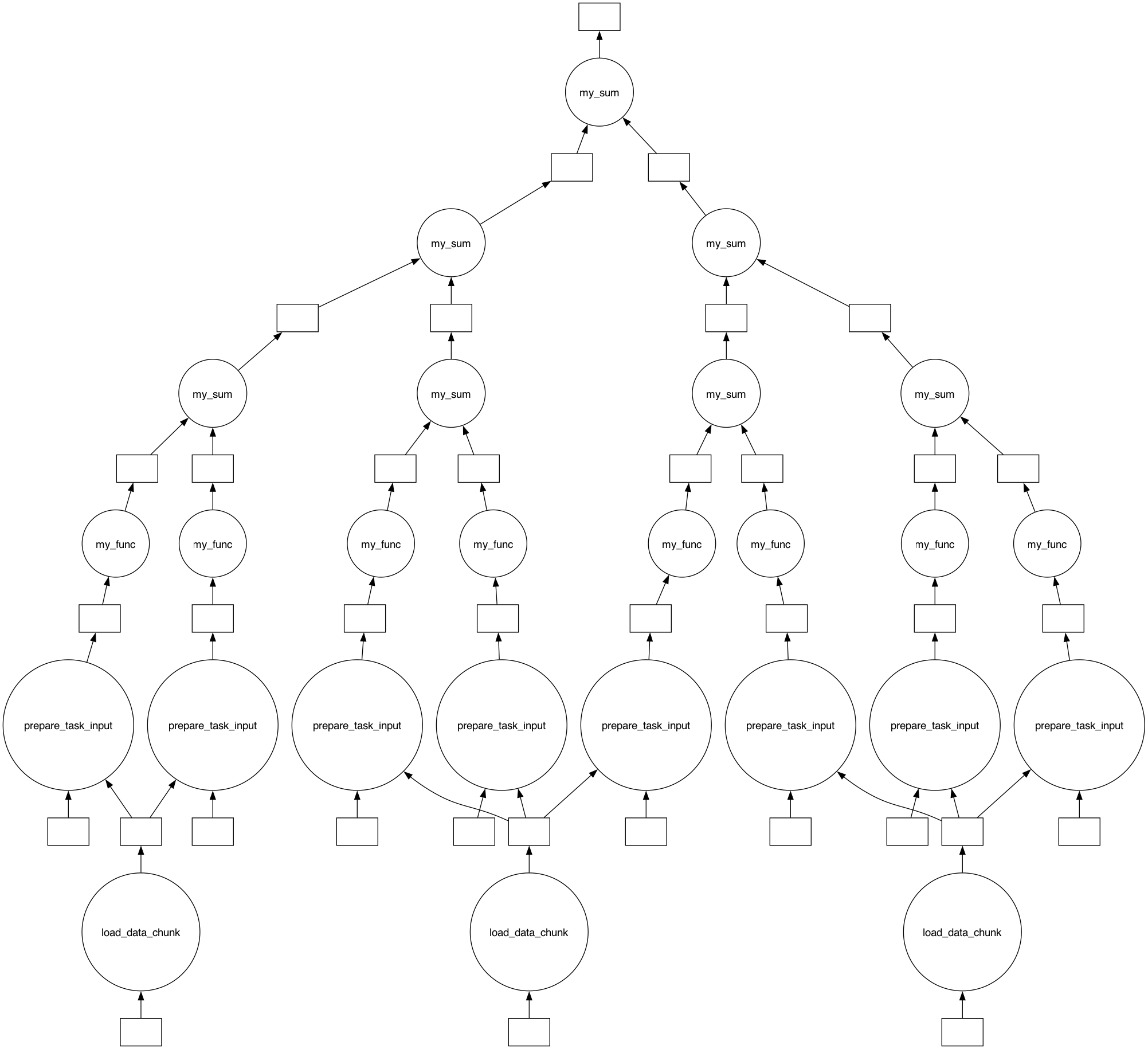
[36]:
result = dask.compute(dask_graph)[0]
print("Result:", result)
Result: 11006957020716.6
Scheduler Plugin
Experimental
For distributed execution, register ViperGraphPlugin with the Dask client before submitting the graph. The plugin reads the viper_load_group and viper_map_pair annotations added by generate_dask_workflow and adjusts task priorities so that:
Only one load group (zarr chunk) is active in memory at a time.
Reduction-adjacent map tasks are scheduled together, allowing the binary tree to collapse results level-by-level with minimal memory overhead.
from toolviper.dask.plugins.scheduler import ViperGraphPlugin
from toolviper.dask.client import local_client

client = local_client(cores=4, memory_limit="8GB")
client.register_scheduler_plugin(ViperGraphPlugin())

# Now submit the graph as usual:
# dask.compute(dask_graph)
The plugin is purely advisory — if it is not registered the graph still computes correctly, just without the optimized scheduling order.
Local Disk Caching
Experimental
Independently of the scheduler plugin, toolviper and the `map <https://graphviper.readthedocs.io/en/latest/_api/autoapi/graphviper/graph_tools/map/index.html#graphviper.graph_tools.map.map>`__ function support caching data to a compute node’s local disk when multiple passes have to be made over larger-than-memory data. Instead of re-reading the same data from a clustered file system or binary object store on every pass, a node task can write the
chunk it loaded to fast node-local storage on the first pass and read it back from there on subsequent passes.
Local caching is enabled by passing the node-local directory to use as the local_dir parameter of the toolviper Dask clients (local_client(..., local_dir=...) or slurm_cluster_client(..., local_dir=...)), or equivalently by setting the VIPER_LOCAL_DIR environment variable before the graph is built:
import os
os.environ["VIPER_LOCAL_DIR"] = "/mnt/nvme/viper_cache"  # node-local storage
When it is set, `map <https://graphviper.readthedocs.io/en/latest/_api/autoapi/graphviper/graph_tools/map/index.html#graphviper.graph_tools.map.map>`__ adds the following items to each task’s input_params (when it is not set, date_time is None and the other keys are absent):
viper_local_dir: the cache directory.date_time: a timestamp identifying the run, so that cached data from different runs is kept apart. It can also be passed explicitly viamap(..., date_time=...)to reuse the cache written by an earlier run.node_ip: a stable task-to-compute-node assignment, so that on repeated passes a task can be routed to the node that already holds its cached data.
GraphVIPER only provides this bookkeeping — the node task itself implements the write-on-first-pass / read-on-later-passes logic under viper_local_dir.
[37]:
toolviper.__version__
[37]:
'0.1.3'